BrainVoyager v23.0
Spatial Transformation Matrices
This topic aims to provide knowledge about spatial transformations in general and how they are implemented in BrainVoyager, which is important to understand subsequent topics about coordinate systems used in BrainVoyager and relevant neuroimaging file formats. The topic describes how affine spatial transformation matrices are used to represent the orientation and position of a coordinate system within a "world" coordinate system and how spatial transformation matrices can be used to map from one coordinate system to another one. It will be described how sub-transformations such as scale, rotation and translation are properly combined in a single transformation matrix as well as how such a matrix is properly decomposed into elementary transformations that are useful e.g. for display purposes. The presented information is aimed towards advanced users who want to understand how position and orientation information is stored in matrices and how to convert transformation results from and to third party (neuroimaging) software.
Note. In the equations used in this chapter, variables representing vectors and matrices are written in bold font (e.g. "M"), whereas scalars are written in italics (e.g. "x").
3D Affine Transformation Matrices
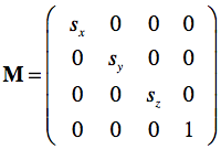
Any combination of translation, rotations, scalings/reflections and shears can be combined in a single 4 by 4 affine transformation matrix:
Such a 4 by 4 matrix M corresponds to a affine transformation T() that transforms point (or vector) x to point (or vector) y. The upper-left 3 × 3 sub-matrix of the matrix shown above (blue rectangle on left side) represents a rotation transform, byt may also include scales and shears. The last column of the matrix represents a translation (blue rectangle on right side). When used as a coordinate system, the upper-left 3 x 3 sub-matrix represents an orientation in space while the last column vector represents a position in space. The transformation T() of point x to point y is obtained by performing the matrix-vector multiplication
The 4 by 4 transformation matrix uses homogeneous coordinates, which allow to distinguish between points and vectors. Vectors have a direction and magnitude whereas points are positions specified by 3 coordinates with respect to the origin and three base vectors i, j and k that are stored in the first three columns. Points and vectors are both represented as mathematical column vectors (column-matrix representation scheme, see note below) in homogeneous coordinates with the difference that points have a 1 in the fourth position whereas vectors have a zero at this position, which removes translation operations (4th column) for vectors. The transformation of the point x to point x' is thus written as x' = Mx or:
For vectors the value in row 4 would be 0 instead of 1 removing the translation operation by multiplying the 4th vector of matrix M by 0. Performing the matrix-vector product multiplies each column vector of matrix M with the corresponding value (x, y, z, 1) of column vector x. and the sum of these four scalar-vector products results in the output vector x'.
We next consider the nature of elementary 3D transformations and how to compose them into a single affine transformation matrix. Note that for an affine transformation matrix, the final row of the matrix is always (0 0 0 1) leaving 12 parameters in the upper 3 by 4 matrix that are used to store combinations of translations, rotations, scales and shears (the values in row 4 can be used for implementing perspective viewing transformations, used e.g. in OpenGL, but this is not needed for the spatial transformations needed in neuroimaging). Homogeneous coordinates (4-element vectors and 4x4 matrices) are necessary to allow treating translation transformations (values in 4th column) in the same way as any other (scale, rotation, shear) transformation (values in upper-left 3x3 matrix), which is not possible with 3 coordinate points and 3-row matrices. Note that separate affine matrices may store individual transformations. With homogeneous coordinates any number and type of elementary transformation stored in its own matrix can be combined in any order by matrix-matrix multiplication resulting in a single transformation matrix.
The Translation Matrix
A translation matrix simply moves an object (e.g. voxels of a volume, vertices of a mesh) along one or more of the three axes. A transformation matrix representing only translations has the simple form:
Applying a translation matrix to a point v reveals that Mv simply adds the translation vector tx, ty, and tz to the components of v (vx, vy, vz) producing translation (shift):
The Scaling Matrix
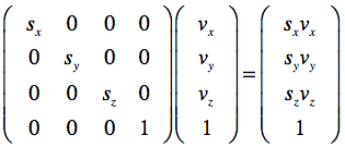
A scaling transform changes the size of an object by expanding or contracting all voxels or vertices along the three axes by three scalar values specified in the matrix. A scaling matrix has the following form:
The sx, sy, and sz values represent the scaling factor in the X, Y, and Z dimensions, respectively. Applying a scaling matrix to a point v produces an output vector with each component multiplied with the corresponding scaling value:
The Rotation Matrix
A rotation matrix rotates an object about one of the three coordinate axes, or any arbitrary vector. The rotation matrix is more complex than the scaling and translation matrix since the whole 3x3 upper-left matrix is needed to express complex rotations. It is common to specify arbitrary rotations with a sequence of simpler ones each along one of the three cardinal axes. In each case, the rotation is through an angle, about the given axis. The following three matrices RX , RY and RZ and represent transformations that rotate points through the angle θ in radians about the coordinate origin:
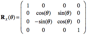
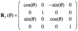
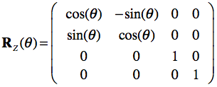
It must be further defined whether positive angles perform a clockwise (CW) or counterclockwise (CCW) rotation around an axis with respect to a specification of the orientation of the axis. In BrainVoyager, positive rotation angles cause a counterclockwise rotation about an axis as one looks inward from a point on the positive axis toward the origin. This is commonly the case for right-handed coordinate systems. Note that transformation matrices containing only rotations and translations are examples of rigid-body (solid-body) transformations, which do not alter the size or shape of an object.
Euler Angles and Quaternions
Euler angles are a set of three angles that represent orientation in space. Each angle represents a rotation around one of three orthogonal axes (for example, the x, y, and z axes). The order of rotations is important because matrix multiplication is non-commutative (see below). Representation of orientations as a set of three angles is intuitive and they are thus used in BrainVoyager's user interface, e.g. in the Coregistration tab of the 3D Volume Tools dialog. However, Euler angles also come with a serious issue called gimbal lock. Gimbal lock occurs when a rotation by one angle reorients one of the axes to be aligned with another axis. Any further rotation around either of the two now-colinear axes will result in the same transformation of the model, removing a degree of freedom from the system. Thus, Euler angles are not ideally suitable for accumulating rotations. A better approach is to construct a unique transformation matrix given an angle and an arbitrary rotation axis. An elegant alternative approach is to use quaternions.
Quarternions offer an alternative way of describing rotations. A quaternion is a four-dimensional quantity that is somewhat similar to a complex number. While a complex number has one imaginary part i next to the real part, a quaternion has a vector component with three imaginary parts, i, j, and k. In the same way as a rotation matrix takes an angle and an axis to rotate around, a quaternion uses the angle as the real part and the axis in the vector (imaginary) part, yielding a quaternion that represents a rotation around any axis. A sequence of rotations can be represented by a series of quaternions multiplied together, producing a single resulting quaternion that encodes the combined rotations. While this can also be achieved with a sequence of matrices representing rotations around the Cartesian axes multiplied together, the matrix method may run into the gimbal lock problem. Quaternions are thus an attractive alternative method to represent rotations because they do not suffer from gimbal lock. Note that it is also possible to convert a quaternion into a 3x3 rotation matrix and vice versa.
The Order of Rotations in BrainVoyager
The default order of rotations in BrainVoyager's internal coordinate system is, of course, X, Y, Z. Since, however the GUI shows "system" coordinates (XSYS: right to left or left to right, YSYS: anterior to posterior, ZSYS: superior to inferior), the order of rotations of angles for the displayed axes is as follows:
- Rotation around YSYS axis (= internal XBV axis)
- Rotation around ZSYS axis (= internal YBV axis)
- Rotation around XSYS axis (= internal ZBV axis)
If three non-zero angles are supplied, BrainVoyager thus performs first the rotation around the YSYS axis (XBV axis), then around the ZSYS axis (YBV axis) and finally around the XSYS axis (ZBV axis). For a complete specification of a rotation, the position of the rotation point (or pivot point) can also be specified around which the data set is rotated. The default coordinates for the rotation point is the center of a volume data set, i.e. (DIM-1.0)/2.0 with DIM equal to the number of voxels in the respective dimension. In a 256 by 256 by 256 data set, the rotation point would be thus 127.5, 125.5, 125.5. If translation parameters are specified, the rotation point changes accordingly because the translation is performed prior to the rotation.
The Shear Matrix
Shear operations "tilt" objects; they are achieved by non-zero off-diagonal elements in the upper 3 by 3 submatrix. A transformation matrix expressing shear along the x axis, for example, has the following form:
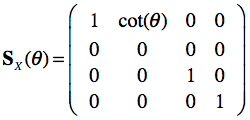
Shears are not used in many situations in BrainVoyager since in most cases rigid body transformations are used (rotations and translations) plus eventually scales to match different voxel sizes between data sets. For MNI normalization of measured volumes, however, a transfromation matrix is calculated that uses all 12 free parameters including shear operations.
Concatenating Transformations
Transformation of a point (or vector) from one space to another involves a simple matrix–vector multiplication operation. Multiplying a point by a sequence of matrices can apply a sequence of transformations. It is not necessary, however, to store the intermediate points after each matrix–vector multiplication. Rather, it is possible and generally preferable to first multiply all of the matrices together to produce a single matrix representing the entire transformation sequence. This matrix can then be used to transform points directly from the source to the destination coordinate space. Forming products of transformation matrices is often referred to as a concatenation, or composition of matrices.
It is important to realize that the order of transformation matrices in a multiplication matters. If, for example, the first transformation rotates an object 45° around the Y axis and the second transformation translates it by 10 units along the X axis, the result is different than if the object is first translated 10 units along the X axis followed by the rotation of 45° around the Y axis. For column-matrix representation of points and vectors (as used in this text), matrices written in a sequence form left to right are actually applied from right to left. Thus an input vector appears on the right side and the sequence of transformations operates in reverse order (from right to left). Thus to first rotate (matrix R) and then translate (matrix T) vertex v, one would write u = TRv.
Note 1. Matrix multiplication is associative. For any three matrices, A, B, and C, the matrix product ABC can be performed by first multiplying A and B or by first multiplying B and C: ABC = (AB)C = A(BC). Therefore we can evaluate matrix products using either a left-to-right or a right-to-left associative grouping. The important point is that matrix multiplication is not commutative in general: The matrix product AB ("A premultiplies B") is generally not equal to BA ("B premultiplies A"). This means that if a sequence of translations, rotations and scalings is applied, the order in which the elementary transformation matrices appear is critical to determine the overall transformation. Only for some special cases, such as a sequence of transformations of the same kind (i.e. two translations or two rotations around the same axis), the multiplication of transformation matrices is commutative.
Note 2. The "right-to-left" order of transformation matrices holds for column-matrix representations as used in this text. In this representation, points such as u and v are represented as column vectors. Another convention being used in the literature is row-matrix representation in which points are represented as row vectors. A conversion between these conventions is easy by exploiting a property of matrix transposition: The transposition of a matrix product is equivalent to the product of the transposition of each matrix, with the order of multiplication re-versed: (AB)T = BTAT . Thus, the transformation of vector v in columnar-matrix representation u = M2M1v equals u = vT M1T M2T in row-matrix representation.
Copyright © 2023 Rainer Goebel. All rights reserved.