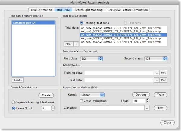
After describing basic principles about SVMs in the last blog, we will discuss now how to actually apply them for fMRI data sets in BrainVoyager QX 2.0. The ROI-SVM tab of the Multi-Voxel Pattern Analysis dialog (see figure above) allows to run SVMs on the data of a selected region-of-interest (ROI) implementing one way of feature selection. The selected ROI can be as big as the whole cortex or as small as a few voxels.

Input 1 - ROI-Based Feature Selection

In order to load a relevant volume-of-interest (VOI) file, use the “Load” button in the ROI-based feature selection field. In the appearing list of VOIs, select the one you want to use for feature selection. In the example snapshot above, the VOI “SomatoRegionLH” encompasses a region in the left hemisphere, which includes somatosensory cortex since the data used in the example presented here is the result of a somatosensory experiment involving repeated stimulation of fingers (D2, D3 and D4).

Input 2 - Single-Trial Response Estimates

This experiment has been used already in the “MVPA Basics” blog entry to describe how single-trial response estimates are obtained from time course (VTC) data. For each VTC file, a volume map (VMP) file is created containing the single-trial estimates (t values, beta values) for each voxel. These VMP files must now be added to the “Trial data” list shown in the snapshot above (if the trial estimates have just been performed, the “Trial data” list is populated automatically).

Generation Of Training and Test Patterns

With the selection of a VOI and one or more single-trial data VMP files, the actual training data for the SVM classifier can be generated by clicking the “Create” button in the “Create ROI-MVPA data” field. If trial estimates for more than two conditions have been generated in the “Trial Estimation” tab, you may now select the two classes that you would like to compare using the “First class” and “Second class” combo boxes in the “Selection of classification task” field. Here we want the SVM to learn to classify whether digit 2 (“D2”) or 3 (“D3”) is stimulated, which is more challenging than using the more distant digits 2 and 4 producing less activation overlap in the somatosensory cortex.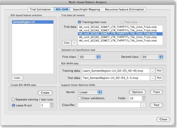


Note that the “Create ROI-MVPA data” step will not only create training data but also data for testing the generalization performance of the trained classifier. There are two options for separating training and test data. If you have several experimental runs and you want to keep apart one (or more) runs for testing, switch to the “Separate training / test runs” option. Then you can fill the trial data list separately with training and test data. After clicking the “Create” button, only the data specified as training runs will be used to generate training patterns, while the data specified as test runs will be set apart for testing purposes. If you decide instead to use a proportion of the trial data from all runs for testing, select the “Leave N out” option in the “Create ROI-MVPA data” field and specify in the respective spin box how many trials you want to randomly extract for testing the classifier. Note that the number entered here will be applied to each class. If the value is set to “5”, 5 trial estimates will be picked out from each class and set aside for testing. The snapshot above shows the “ROI-SVM” tab after clicking the “Create” button using the “Leave N out” option with N=5. The training and test data has been created and the corresponding output files are shown in the “ROI-MVPA data” field. The name of the files describe what they contain, e.g. the “Learn_SomatorRegion-LH_D2-D3_40-40.mvp” file name indicates that this MVP file contains 40 patterns for class “D2” and 40 patterns for class “D3” and that the patterns are defined over the voxels (features) of the “SomatoRegion-LH” ROI. The name of the file containing the test patterns “Test_ SomatorRegion-LH_D2-D3_5-5.mvp” indicates that it contains 5 patterns per class as requested with the “Leave N out” option. If you want to know which patterns have been moved to the test pattern, have a look in the “Log” pane. In the example, the following lines have been printed in the log:

No of all training data trials for class1, class2: 45 45
Class 1 trials removed for testing: 18 43 19 78 38
Class 2 trials removed for testing: 67 34 29 47 31

The format of the generated MVP files has been described in the previous blog entry. Instead of two features used there, each pattern now contains about 1500 entries, which is the number of voxels in the specified “SomatorRegion-LH” ROI. You may visualize the training and test patterns by clicking the respective “Plot” button in the “ROI-MVPA data” field. Note that if you want to run another classifier on the same data, you need not to re-create the ROI trial data but you can the Brows (“...”) buttons to select MVP files.

SVM Model Selection

We can now train a support vector machine on the patterns stored in the file shown in the “Training data” text field by clicking the “Train” button. This would use a SVM with default settings including a linear kernel and a value of “1” for the penalty parameter “C”. While it is possible to select a non-linear kernel using the “Kernel” combo box in the “Support Vector Machine (SVM)” field, we recommend to stick to the default linear kernel since this allows us to use the weight vector of the trained SVM for visualization and feature selection. As described in the previous blog, a linear kernel is also recommended for fMRI data, which can be assigned to the “many features, few patterns” case.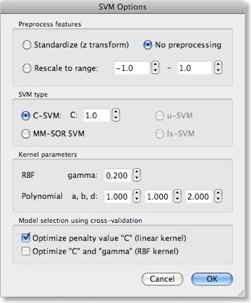


While using a linear kernel is appropriate, it is important to optimize the C parameter to create a classifier with good generalization performance (influencing the size of the margin). As described in the previous blog, a good model selection technique combines systematic parameter search with n-fold cross-validation. To enable this technique, invoke the “SVM Options” dialog by clicking the “Options” button in the “Support Vector Machine (SVM)” field. The first field in this dialog, “Preprocess features”, allows to standardize or rescale the data of a feature across the available patterns. This is important in case that the different features have very different variances, but it is normally not necessary when using z normalization during the trial estimation step. The “SVM type” field allows to set a desired value for the “C” parameter for SVM training. We will, however, turn on the “Optimize penalty value “C” (linear kernel)” option in the “Model selection using cross-validation” field, which will systematically test values for “C” in a wide range.

SVM Training

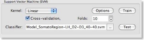
After clicking the “OK” button, make sure that the “Cross-validation” option is also turned on in the “Support Vector Machine (SVM)” field of the “Multi-Voxel Pattern Analysis” dialog and set a value for the number of folds (or keep the default value “10”). To run the model selection process, click the “Train” button. Since we turned on parameter optimization with cross-validation, a series of SVMs with different C values will be generated and the test performance of each model will be evaluated using cross-validation. The “Log” pane will inform about the progress with the following output (only a subset of the printed lines are shown):

Testing parameter C=0.00673795 with 10-fold cross validation - Accuracy: 92.5%
Testing parameter C=0.011109 with 10-fold cross validation - Accuracy: 91.25%
:
Testing parameter C=1.64872 with 10-fold cross validation - Accuracy: 91.25%
Testing parameter C=2.71828 with 10-fold cross validation - Accuracy: 93.75%
Testing parameter C=4.48169 with 10-fold cross validation - Accuracy: 91.25%
:
Testing parameter C=1.2026e+06 with 10-fold cross validation - Accuracy: 88.75%
Testing parameter C=1.98276e+06 with 10-fold cross validation - Accuracy: 91.25%

Setting C to value resulting in best generalization performance: C=2.71828

Running SVM with C=2.71828 and linear kernel

After evaluating SVMs with different C parameter values, the program decides on using the value C=2.7, which produced the highest cross-validation accuracy (93.75% correct classification). Using the whole training data, it runs a final SVM training process with this C value. The performance on the training data is also plotted in the “Log” (only the prediction output of the last 20 of all 80 patterns is shown):

:
1.00036 1
1.23035 1
0.99963 1
1.00025 1
1.00006 1
0.999548 1
1.09946 1
1.16695 1
-1.00018 -1
-1.00031 -1
-0.999842 -1
-0.999998 -1
-1.19388 -1
-1.00022 -1
-1.04356 -1
-1.00034 -1
-0.9996 -1
Accuracy (full training set): 100%

The left column shows the predicted value and the right column the “label” indicating to which class the respective pattern actually belongs (“1” class 1, “-1” class 2). The trained SVM model is saved in a “SVM” file allowing to re-use the classifier in the future. The name of the stored SVM file is shown in the “Classifier” text box within the “Support Vector Machine (SVM)” field. In the snapshot above, the obtained SVM file is “Model_SomatorRegion-LH_D2-D3_40-40.svm”; the created file name is derived from the name of the used training data allowing to identify the “MVP” data belonging to the “SVM” modelt. The trained SVM can now be used to classify the test data, which was not used during model selection. When pressing the “Test” button, the data contained in the file shown in the “Test data” text box of the “ROI-MVPA data” field will be used as input for the trained SVM shown in the “Classifier” text box of the “Support Vector Machine (SVM)” field. After pressing the “Test” button, the predicted values fort the 10 test cases of our sample data are printed in the “Log”:

SVM output - predictions (plus targets) for test exemplars:
0.476441 1
0.990862 1
0.79285 1
1.16716 1
0.545607 1
-0.618332 -1
-0.299141 -1
-0.557493 -1
-0.0442947 -1
-0.576111 -1
Test data - prediction accuracy (assuming labels are known): 100%

This result shows that the classifier has indeed learned how to weight the voxels (features) of the ROI to discriminate between the two classes also for unseen test cases. While a performance of 100% is impressive, the results will be less good when less cases are used for learning and, hence, more cases are used for testing. In order to test, for example, the performance when setting 33% of the 45 trials per class for testing (instead of 11% or 5 cases), set a value of 15 in the “Leave N out” spin box and rerun the described steps.

Visualizing the Weight Vector

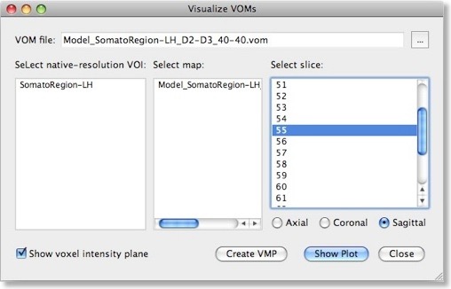
The weights of a trained SVM together with the bias term define the discriminant functions of the classifier (see previous blog). In case of a linear classifier, the absolute value of a weight can be interpreted as the strength of contribution of the respective voxel to the multivariate classification. It is thus useful to visualize the weights of the involved voxels to obtain a “SVM map”, which aids in making the “machine learning black box” more transparent. Visualizing the weights requires the knowledge which voxel (i.e. the respective x, y, z coordinates) corresponds to a specific weight, This link is lost when the MVP data file is created since this file only stores the estimated trial response values per voxel, but not the voxels’ coordinates. To keep that link alive, BrainVoyager actually saves a special “VOM” (volume-of-interest map”) file to disk containing the coordinates of each ROI voxel. The link to the MVP data and SVM weight vector is kept alive since the VOM file presents the coordinates of voxels in the same order as used in the MVP and SVM weight vector. While a VOM file is saved already during creation of the MVP data, the weight values are added after training the classifier. To visualize the weight vector of a SVM, use the “Visualize VOM” dialog, which can be launched from the “Options” menu. The Browse button (“...”) in the top part of the dialog allows to select the desired VOM file, which has the same name as the trained SVM except that the extension is changed from “.svm” to “.vom”.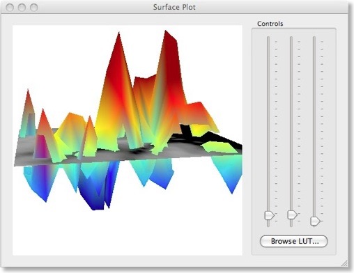

There are two different ways to visualize the weights over the corresponding voxels. One way presents the weights in a 3D plot for selected axial, coronal or sagittal slices (see snapshot above). This view allows to inspect in great detail how the weights are spatially distributed. You can drag the mouse within the plot perform rotations or use the sliders on the right side. It is also possible to change the color look-up table by using the “Browse LUT” button.

Another option to visualize the weights is in form of a standard volume map (see snapshot below). This can be achieved directly from the “Visualize VOM” dialog by clicking the “Create VMP” button. Note that the map is in “native resolution”, i.e. in the same resolution as the original VTC data and not in anatomical resolution (except if the VTC data has the same resolution). To ensure that the whole SVM analysis is based on native resolution data, the VOI used during the MVP data creation step is actually transferred from high-resolution (1 VOI voxel = 1 anatomical voxel) to the resolution of the VTC data. If the VTC data is represented in resolution “2” or ”3”, 1 functional voxel equals 2 x 2 x 2 / 3 x 3 x 3 anatomical voxels. Only after this transformation has been done, the trial estimates of the VTC data are linked to the VOM voxels keeping native resolution.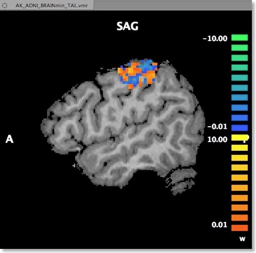


An advantage of visualizing the weight vector as a volume map is that it can be thresholded allowing to quickly check for the most relevant voxels by increasing the threshold. Since the weights may be very small when having several thousand features, the weight values are scaled when creating the new “w” (weight) map type (see snapshot above). The scaling process maps the values in the range from 0 to the maximum absolute value to a range from 0 to 10.

This completes the description of the ROI-SVM tools in BrainVoyager QX 2.0. The next blog entry will describe the new “Movie Studio” that allows to create stunning animations. We will then return to the machine learning tools and I will describe how an important technique, recursive feature selection, can be used to find the most discriminative voxels within large brain regions.