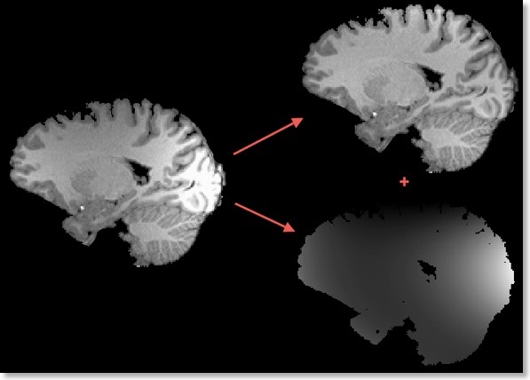
Intensity inhomogeneities in MR images can substantially reduce the accuracy of segmentation and registration. Despite advances of correcting spatial intensity inhomogeneities, the advent of multichannel phased array coils and 7T+ scanners have increased (again) the importance of this problem for post-scan processing (see image on left side in figure at top). Since many years, BrainVoyager includes a powerful intensity inhomogeneity correction (IIHC) tool that is based on a “surface fitting” approach to voxels preliminary labelled as white matter. This tool required, however, that presumed white matter voxels were manually selected (“pre-segmented”) and this could be time-consuming and the resulting quality depended on the experience of the user.

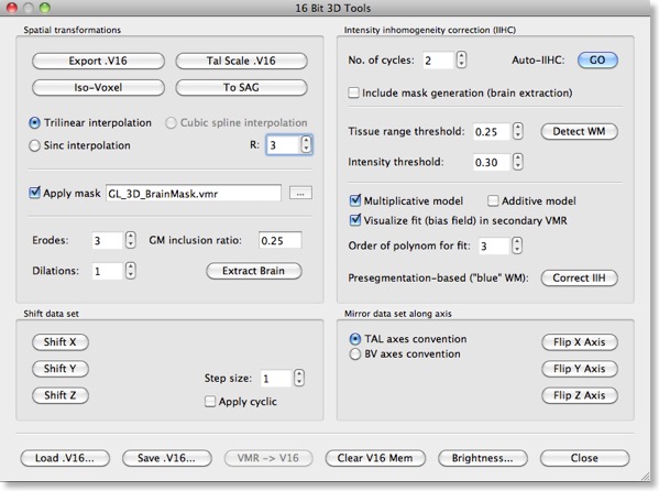
Version 2.2 of BrainVoyager QX introduces a new IIHC tool that operates fully automatic and produces excellent results. It is based on the same “surface fitting” approach as in previous versions that compare well with other IIHC tools (e.g. Sled et al., 1997, A comparison of retrospective intensity non-uniformity correction methods for MRI. Lecture Notes in Computer Science). The new version includes, however, several new tools, including automatic white matter labeling and integrated brain extraction. In most cases, pressing the “GO” button in the “Intensity inhomogeneity correction (IIHC)” field of the updated “16 Bit 3D Tools” dialog (see figure below) is sufficient to create a homogeneous data sets in a few seconds. Starting automatic IIHC triggers a sequence of processing steps resulting in a segmented, homogeneous brain data set (see top right image in figure above). In addition to the inhomogeneity corrected VMR data set, the automatic procedure also generates a representation of the “bias field” in the secondary VMR. This bias field is the fitted model of the low-frequency intensity variations of automaticaly labeled white matter voxels over space (see bottom right image in figure above).

While a single run of the automatic IIHC process leads to very good results, the process is repeated once as default (No. of cycles: 2) to further increase the resulting homogeneity. More than two iterations do usually not lead to significant further improvements as can be assessed with the displayed intensity histograms that are generated for each iteration (see figure below). Each histogram shows the result before (blue line) and after (yellow line) application of one cycle through the processing pipeline. In the plot on the left side below (iteration 1), the blue line indicates that white and grey matter voxel intensities overlap substantially since there is only one major peak in the histogram; the yellow line indicates the successful application of the automatic inhomogeneity correction process since clearly revealing two peaks.

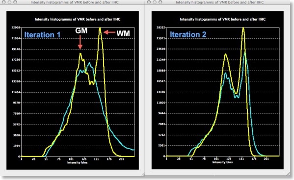
The plot on the right (Iteration 2) shows that a second run through the IIHC tool leads to further improvements but they are no longer as substantial than those obtained for the first iteration. Additional iterations do not usually not enhance the separation of the two peaks any further.
Note that the bias fields calculated at each iteration are also stored to disk. Since the first bias field highlights the most severe inhomogeneities, it is shown in the secondary VMR view even when running multiple iterations. Bias field visualizations from subsequent iterations can be loaded as separate VMRs or loaded in the secondary VMR view. More details about the automatic intensity inhomogeneity correction tool can be found in the BrainVoyager QX User’s Guide.