BrainVoyager v23.0
Pairwise Source to Target Alignment
After having created the standard sphere (SPH) curvature maps of at least two hemispheres, one can start the alignment procedure. In the most simple way, BrainVoyager allows to specify a source and a target mesh for a curvature-driven pairwise alignment. The explicit pairwise procedure described here requires manual interaction to perform sub-stages of alignment and is mainly recommended for gaining insights in the involved processes. For alignment of (large) groups of cortex hemispheres, the group alignment approach is recommended that runs in an automatic way. The explicit pairwise alignment is also useful when one wants to bring information from an atlas cortex hemisphere, e.g. parcellation schemes, to an individual hemisphere mesh.
Creating a Target Spherical Curvature Map
The first step of the explicit pairwise source-target CBA consists of preparing the curvature map of one individual hemisphere as the target curvature to which one or more other hemisphere meshes can be aligned subsequently. This preparatory step converts a normal vertex-based curvature surface map (SMP) file into a representation using a spherical coordinate system, which is called a spherical map (PMP) file. A spherical coordinate system is used for alignment since it is indpendent of the number of vertices used in the surface maps and because it is easier to calculate relative vertex movements during alignment in a 2-dimensional coordinate system of longitude and latitude angles.
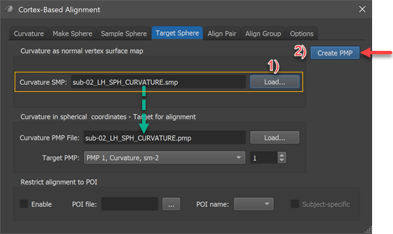
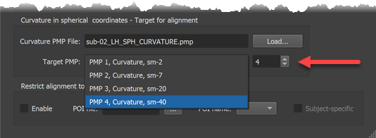
The conversion into a spherical coordinate system is performed in the Target Sphere tab of the Cortex-Based Alignment dialog (see screenshot above). The surface map of the subject's hemisphere that should serve as a target ("sub-02_LH_SPH_CURVATURE.smp" in the example) needs to be loaded in the Curvature SMP field by using the corresponding Load button in the Curvature as normal vertex surface map field (see step 1 above). The conversion process is then performed by clicking the Create PMP button. The program will create a standard sphere (SPH) mesh, loads the provided curvature map and then maps the curvature values from vertex (Euclidean) coordinates (3 values) into a polar coordinate system (2 values). The created file ("sub-02_LH_SPH_CURVATURE.pmp" in the example) is finally saved to disk and appears also in the Curvature PMP file field in the Curvature in spherical coordinates - Target for alignment field. In case one wants at a later stage reuse an already created PMP file, one can simply reload the file using the respective PMP Load button. As can be revealed by clicking on the Target PMP box, the PMP file contains 4 sub-maps representing curvature at various smoothing levels in the same way as the original curvature SMP file.
Aligning Source Curvature to Spherical Target Map
For the second step of the explicit pairwise source-target CBA the standard curvature (SMP) map file of another subject needs to be specified in the Align Pair tab.
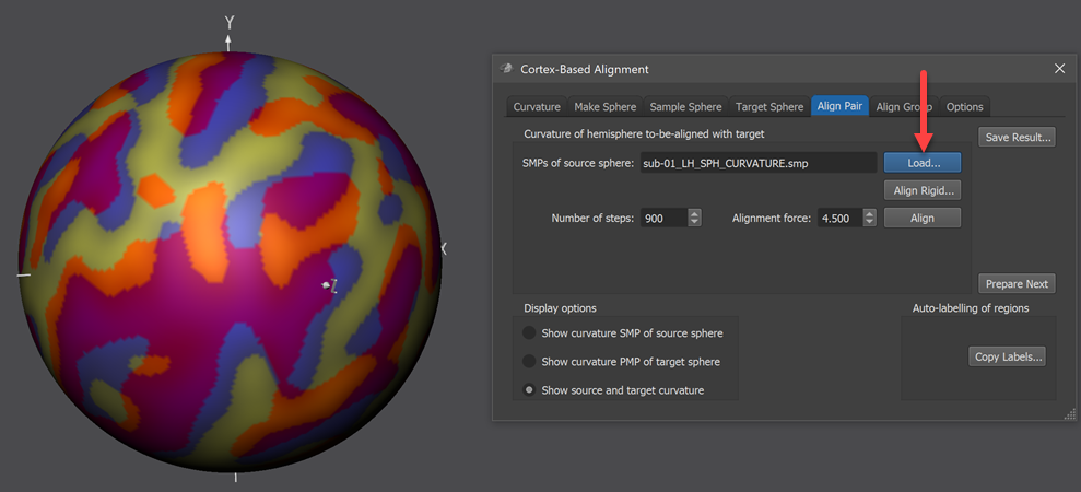
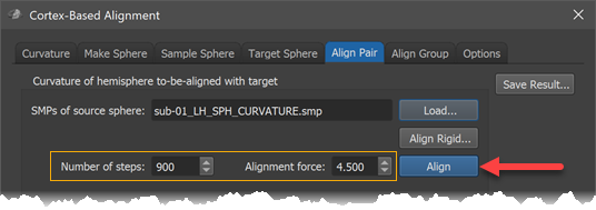
The curvature SMP file of the source hemisphere need to be loaded using the Load button on the right side of the SMPs of source sphere field located in the Curvature of hemisphere to-be-aligned with target field (red arrow in screenshot above). The standard sphre shown in the 3D Viewer will now show information from both the source and target curvature map superimposed (left side in screenshot above). The displayed colors indicate how well the two meshes are aligned at this stage, i.e. before starting CBA. In order to understand the colors involved, the items in the Display options field of the Align Pair tab allow to separately show the colors of the source (Show curvature SMP of source sphere option), target (Show curvature PMP of target sphere option) as well as the combined colors of source and target (Show source and target curvature option, default). The figure below shows the various options for the source and target curvature maps used in this example (data from functional atlas project).
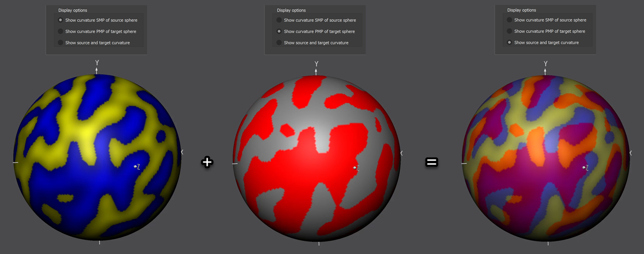
From this figure it should become clear that an optimal (ideal) alignment would contain only pink and light yellow colors indicating perfect overlap of concave (pink = average of blue and red colors indicating "sulci" on "sulci" overlap) and convex (light yellow = average of yellow and grey colors indicating "gyri" on "gyri") curvature. Due to idiosyncratic differences between folding patterns from different subjects, such an ideal case will not be reached but an increase of pink and yellow areas and a decrease of orange (average of yellow and red colors indicating "gyri" on "sulci" overlap) and light blue areas (average of blue and grey colors indicating "sulci" on "gyri" overlap) during CBA will visually indicate successful alignment.
Optional: Rigid Sphere Alignment
While CBA usually enhances correspondence without explicit specification of landmarks, it is, however, important to start CBA at a stage where sulci and gyri are already close to each other on the sphere. In case that major gyri and sulci of hemisphere meshes from different brains deviate very much from each other (despite initial ACPC, MNI or Talairach normalization) sub-optimal alignment results could be obtained. In order to reduce the likelihood of partial mis-alignments, BrainVoyager offers the possibility to run a rigid sphere alignment step prior to locally operating main process. In this "rigid" alignment step, the source sphere is rotated in a specified range of values and the global curvature alignment error with the target curvature map is recorded for each parameter set (rotation values around three axes). The parameter set producing the best fit (smallest alignment errror) will be selected and used to perform a rigid pre-alignment step before starting the CBA procedure. While this step is not an absolute guarantee for avoiding mis-alignments, the likelihood to get optimal results is substantially improved after performing this step.
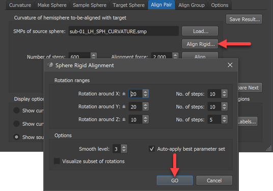
Note that the Auto apply best parameter set option should be turned on (default) in order to prepare a better starting point for the subsequent (non-rigid) alignment step.
Coarse-to-Fine Iterative Alignment
The main alignment process calculates for each vertex on the source sphere small movement steps in a direction that minimizes the difference in curvature assesed at the source vertex and at the corresponding position at the target sphere. These small movements are repeated in an iterative coarse-to-fine fashion. The process can be controlled by using the Target PMP box in the Target Sphere tab. The screenshot below shows selection of the coarsest curvature map (PMP 4, curvature smoothed with 40 iterations). Alternatively one can use the Target PMP spin box (see red arrow below) to select a smoothing level.
After selecting the smoothing level in the Target Sphere tab, the alignment process can be started by clicking the Align button in the Align Pair tab (see arrow in screenshot below). Before clicking the button, one can adjust the preset number of iterations and alignment force by changing the Number of steps value and the Alignment force value but it is recommended to keep the default settings that will be adjusted for each smoothing level automatically.
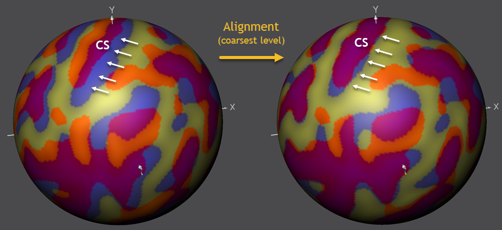
The figure below shows the state of the alignment before and after running CBA using the most smooth curvature maps. It can be seen that large sulci are moved in much better coregistration. The figure highlights the alignment progress for the central sulcus (CS, see below), which overlaps nearly perfectly between the source and target brain after this alignment step.
To continue the alignment process, the next (less smoothed) level needs to be selected in the Target Sphere tab (PMP 3) followed by another click on the Align button in the Align Pair tab. After the second phase of alignment has been completed, these steps should be performed also for the two remaining (PMP 2 and PMP 1) curvature levels in order to complete the process. The screenshot below shows the situation at the begin and end of the most fine-grained (PMP 1) curvature level.
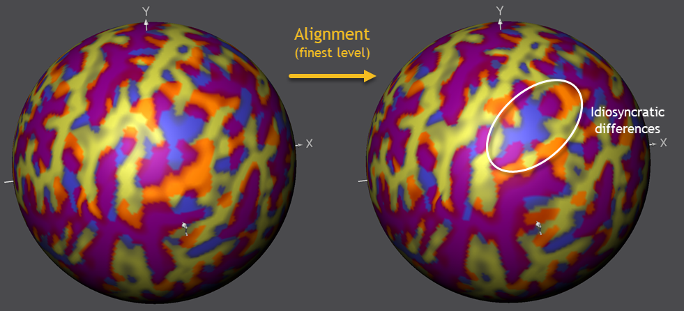
As can be seen on the right side in the screenshot above, most regions have been aligned very well between the source and target hemisphere. Note that regions with a "wrong" overlap (blue or orange colors) will likely reflect fundamental idiosyncratic differences between the macroanatomical characteristics of the included brains that can not be aligned at a fine-grained level. This points to the possibility to use CBA results to guide systematic investigations of such idiosyncratic differences. The figure above highlights a region in the inferior parietal lobule where such idiosyncratic diferences are often observed.
It is important to realize that the alignment at the fine-grained level shown above only reveals what has been added in the last phase, i.e. it builds on the achieved alignment performed when using less smoothed curvature maps. To make this more clear and to show the oevall achieved alignment, the figure below shows the state of overlap before running CBA (left side) and after running CBA (right side).
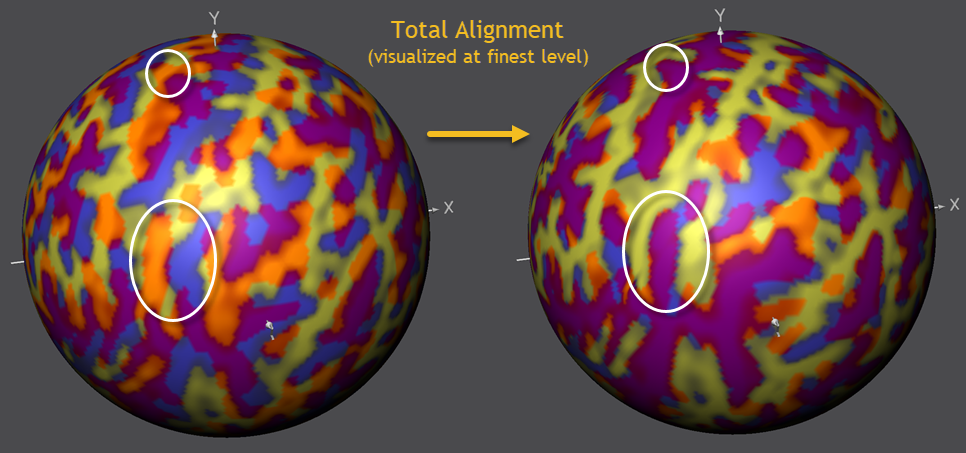
The figure above reveals that the gradual coarse-to-fne alignment approach has aligned not only the "big" sulci and gyri but also more fine-grained sub-sulci inside larger macro-anatomical structures (see circles above highlighting some example cases in the example). Starting the alignment at a fine-grained level would likely not be able to reach such high-quality end results since fine-grained regions would not overlap enough.
In order to save the established alignment, the Save Result button in the Align Pair tab needs to be clicked. The program will then first save the morphed sphere mesh to disk suggesting a name reflecting the source and target hemisphere (e.g. "SUB-01_LH_SPH_ALIGNED_TO_sub-02.srf" in the example). The program will then resample the morphed (aligned) sphere from a generic standard sphere resulting in a sphere-to-sphere mapping (SSM) file describing the displacement of each vertex (e.g. "SUB-01_LH_SPH_ALIGNED_TO_sub-02.ssm" in the example). The created SSM file allows to bring information from the source hemisphere (e.g. statistical maps, time courses, vertex coordinates of folded SPH mesh) into corresponding locations of the target hemisphere. When extending the alignment to multiple subjects, the SSM files from each source brain will thus be transformed into a common target space, which can be an individual brain (e.g., from a group of aligned subjects), a specific (atlas) brain or a representative average group brain. For some applications also the inverse transformation of information is needed, i.e. when one wants to transfer a parcellation scheme from an atlas brain to a source brain. For this purpose, the program will also save a .SSM file ending in the substring "_inv.ssm" (e.g. "SUB-01_LH_SPH_ALIGNED_TO_sub-02_INV.ssm" in the example).
Copyright © 2023 Rainer Goebel. All rights reserved.