BrainVoyager v23.0
Temporal High-Pass Filtering
Voxel time courses of fMRI data often show low-frequency drifts, which is thought to be caused by physiological noise as well as by physical (scanner-related) noise. If not taken into account, these signal drifts reduce substantially the power of statistical data analysis. They also invalidate event-related averaging, which assumes stationary time courses, i.e. time courses with a constant signal level. Because of the clear negative effects for fMRI data analysis, the removal of low-frequency drifts is one of the most important preprocessing steps and should be always performed. Unfortunately, this preprocessing step is also one of the more "dangerous" ones, because condition-related signal changes may also be removed if not properly applied. A good understanding of how high-pass filtering works is, thus, very important.
Since the signal drifts are slowly rising and falling, these drifts are removed by using a high-pass filter. As the name suggests, such a filter lets high frequencies pass (containing stimulus-related activity), but removes low frequencies, i.e. the signal drifts. The following snapshots show typical examples of signal drifts, which are taken from the "OBJECTS" sample data set.
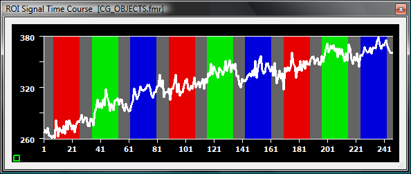
The first snapshot shows an example of a linear drift (voxel position- slice: 18, x: 27, y: 52):
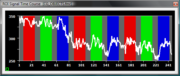
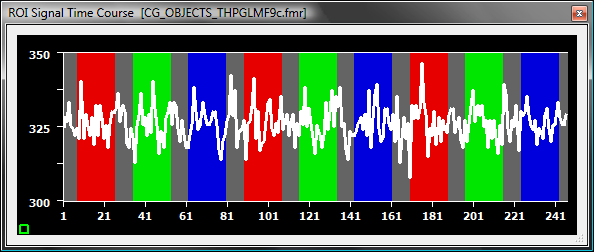
The next snapshot shows an example of a non-linear drift (voxel position- slice: 5, x: 23, y: 48):
To remove the low-frequency drifts, two main options exist:
- The low frequency drifts are removed from each voxel's time course as a preprocessing step. Subsequent processing stages, e.g. statistical data analysis and event-related averaging, can proceed with the "cleaned" data. This approach is described in this chapter.
- The low frequency drifts are not removed during preprocessing, but are modeled as confounding effects during statistical data analysis. This removes the drifts implicitly during calculation of a General Linear Model (GLM). While this approach is statistically elegant, other processing routines, including event-related averaging, can not be performed since the data time courses still contain the drifts (unless one keeps two differently preprocessed versions of the same data). This approach is described in section Adding High-Pass Filter Confound Predictors in the context of statistical data analysis with the General Linear Model.
High-pass filtering is performed separately for the time course of each individual voxel since neighboring voxels can exhibit very different drifts. To apply a high-pass filter during preprocessing of FMR projects, Temporal filtering must be enabled in the Preprocessing options field of the FMR Preprocessing dialog. Since high-pass filtering is so important for fMRI data, this option is turned on as default. For fine-tuning, you may select further options in the Temporal filtering field, which is only visible after clicking the Advanced >> button. You will see that the High-pass option in this field is turned on.
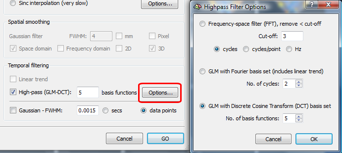
The program offers two major choices. First, the method for high-pass filtering can be selected, and second, the "amount" of filtering can be specified. While the latter setting can be made right in the Temporal filtering field, the method of filtering can only be selected in the High-Pass Filter Options dialog (see snapshot above), which can be invoked by clicking the Options button in the field. Three high-pass filtering methods are offered in the High-Pass Filter Options dialog: 1) high-pass filtering using fourier analysis, 2) high-pass filtering using a GLM approach with a design matrix containing a Fourier basis set (sines and consines), and 3) the same GLM approach, but with a different design matrix with a set of predictors called the Discrete Cosine Transform (DCT). Note that all three methods normally produce very similar results (see below for examples), but different people may have different preferences since there might be slight differences in special situations.
High-Pass Filtering Using Fourier Analysis
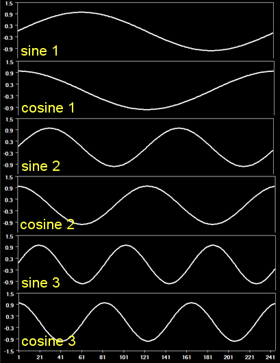
When the Frequency-space filter (FFT) option is chosen, the time course of a voxel is transformed into the frequency domain by application of a fast fourier transform (FFT). In this domain low frequencies can simply removed by setting their values to zero. The data is then transformed back in the time domain, which will then no longer possess the removed low frequencies. The "amount" of filtering can be specified in the Cut-off field in the High-Pass Filter Options dialog or in the Cut-off field in the main dialog. Note that the specified cut-off value means that all frequencies below that value will be removed; if, for example, a value of "3" is given (the default), frequencies "1" and "2", but not "3" will be removed from the data. The cut-off value is normally specified in cycles: A cycle means that one sine wave (from 0 to 360 degrees or 0 to 2PI) is spread across the number of time points of the fMRI data, a cycle of 2 means that two sine waves fall within the extent of the data, and so on. In Fourier analysis, each frequency is actually represented not with just a sine curve, but also a cosine curve, which is a sine curve shifted by 90 degrees (PI/2). The following image shows the sines and cosines for frequencies 1 - 3 as defined for a voxel's time course:
A Fourier analysis estimates the presence of a frequency (potentially contributing to a drift) with two values, one for the sine and one for the cosine curve. These two values can then be used to determine how strong the respective frequency is present in the data, i.e. its amplitude. Another value, the phase can also be calculated from the estimated values for the sine and cosine indicating the "shift" of the sine curve (at which degree it begins at time point 1); while phase values are interesting for several applications, for the purpose of filtering, it is only important to realize that the presence of each frequency is estimated in the data and that frequencies below the cut-off value are removed.
Since FFT-filtering does not work well for purely linear trends, BrainVoyager first applies a linear trend removal step before running the Fourier analysis. A linear trend is estimated by fitting a line through the data estimating its slope and intercept. When the combined linear trend and FFT-based high-pass filter with a cut-off of 3 is applied to the example voxel time courses shown above, the filtered time courses look as follows:
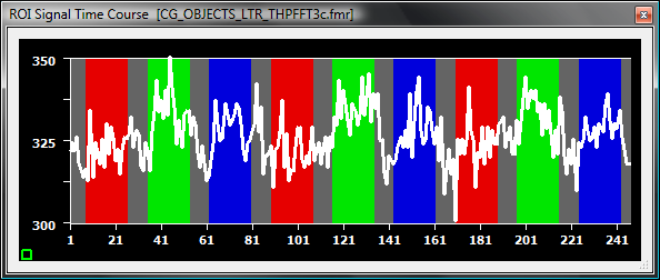
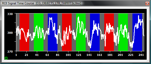
The upper curve is the one originally showing a linear trend, while the lower curve is the one originally exhibiting a non-linear trend. As is readily apparent, both types of drifts have been successfully removed from the data. The name of the resulting preprocessed FMR project will contain the substring "LTR_THPFFT[N]c" (THP = temporal high-pass, FFT = fast fourier transform, c = cycles), where "[N]" will be replaced with the selected cut-off value. The cut-off value can not only be specified as cycles per time course, but also as cycles per point and in Hz. If you select the cycles/point or Hz option in the High-Pass Filter Options dialog, the value corresponding to the cycles per time course will be calculated and shown in the input field. Since cycles per point and Hz must be entered with small values (e.g. 0.006 Hz for a cut-off of 3 cycles), we recommend to enter the cut-off value using the cycles option; furthermore, entered cycles per point or Hz values will internally always computed to a integral cycles value to determine the cut-off value. If the filter is specified as cycles per point, the substring in the filtered FMR data will be "LTR_THPFFT[N]cp" (cp = cycles per point); if specified in Hertz, the substring will be "LTR_THPFFT[N]Hz".
High-Pass Filtering Using GLM Approach with Fourier Basis Set
When the GLM with Fourier basis set option is chosen in the High-Pass Filter Options dialog, the presence of low frequencies are also estimated and removed using sines and cosines, but the filtering is not performed in the frequency domain but in the time domain, i.e. the domain of the originally measured data. The General Linear Model (GLM) is used to estimate the contributions of low frequencies in a voxel's time course (for details on how the GLM works, see topic The General Linear Model). A GLM requires a design matrix containing a set of predictors; for each predictor, the GLM estimates a beta value for in such a way that the sum of predictors, weighted by these betas, produces a predicted time course, which is as close as possible to the measured time course (in the least squares sense, see The General Linear Model). The performance of a GLM to fit a time course depends on the predictors provided in the design matrix. In order to filter low frequency drifts, a design matrix is created containing sines and cosines for low frequencies. The figure with the sine cosine waves shown above represents a design matrix consisting of sines and cosines for 1 - 3 cycles. The number of sine/cosine pairs of such a Fourier basis set can be specified in the No. of cycles input field of the High-Pass Filter Options dialog, or in the respective field in the FMR Preprocessing dialog. In addition to the sine/cosine predictors, a linear trend predictor is added to the filtering design matrix as well as a "constant" (consisting o values of 1.0 for all time points). The predicted time course from a GLM with this design matrix will then be subtracted from the original data resulting in a filtered time course containing only frequencies above those in the design matrix.
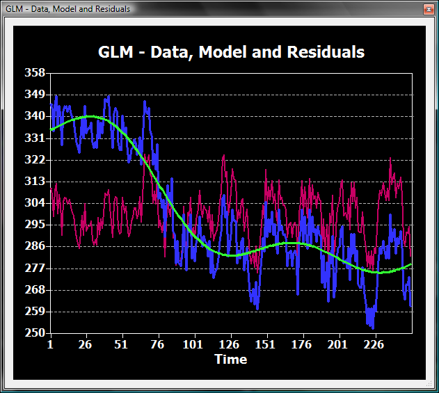
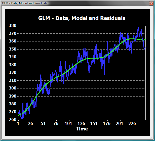
The following snapshot shows the original data in blue (example time course shown also above exhibiting mainly a linear trend) and the fit of the GLM (2 sine/cosine predictors plus linear trend and constant) in green.
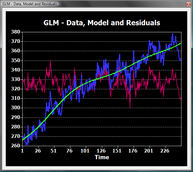
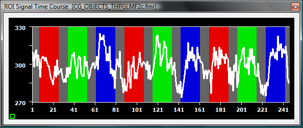
The magenta curve is the difference of the blue and the green curve. While in a "statistical" GLM the magenta curve is considered "noise" (unexplained variation, residuals), it is used as the new voxel's time course in the context of high-pass filtering. This can be readily seen when comparing the magenta curve above from a voxel GLM analysis with the time course of the same voxel from the preprocessed data below.
The snapshot below shows the beta values estimated for each predictor. As expected, the linear trend shows the largest value, but also the sine cosine predictors contribute in explaining the time course drift.
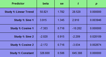
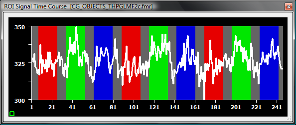
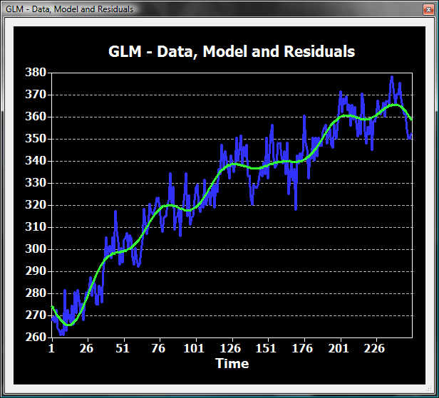
The snapshot below shows the result of the GLM fit (green curve) for the example time course exhibiting a non-linear drift.
The magenta curve, the difference of the blue and green curve, represents the new voxel's time course as can be seen in the snapshot below showing the time course of the respected voxel in the preprocessed FMR data.
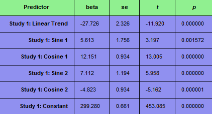
The beta values table below shows that the linear trend predictor contributes strongly also in this case, but the sine and cosine predictors now show much larger values than in the case of a mostly linear trend. The beta weight of cosine 1 is especially strong, which reflects that the time course falls of from initially high values roughly in the shape of a cosine with one cycle in the first part of the time course.
When the GLM Fourier method is used for high-pass filtering, the name of the preprocessed FMR project will contain the substring "THPGLMF[N]c" (THP = temporal high-pass, GLM = general linear model, F = Fourier basis set, c = cycles), where "[N]" will be replaced with the selected number of sine/cosine pairs.
High-Pass Filtering Using GLM Approach with DCT Basis Set
When the GLM with Discrete Cosine Transform (DCT) basis set option is chosen in the High-Pass Filter Options dialog, the presence of low-frequency drifts is also estimated and removed using the GLM approach, but the design matrix will be created not from a Fourier basis set but from a similar alternative, called the Discrete Cosine Transform (DCT). A design matrix with 5 DCT predictors looks like this:
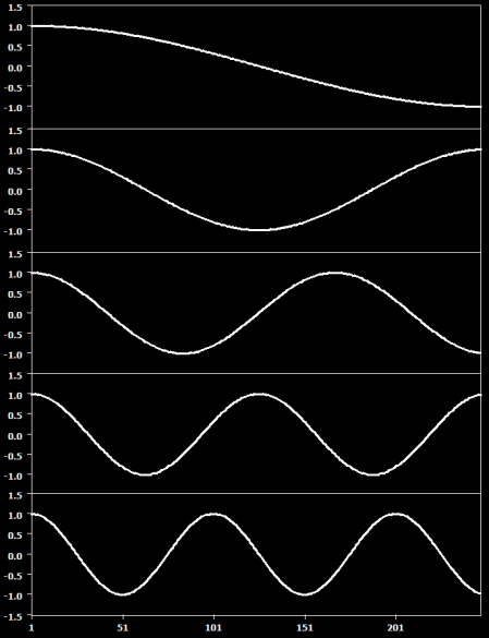
Such a design matrix roughly corresponds to a Fourier basis set with 2 sines and cosines (i.e. two cycles per time course). It is not necessary to add a linear trend predictor to the DCT basis set since the DCT predictors can be combined with appropriate beta values to fit a linear trend; only the constant predictor will the added to the design matrix. The number of DCT basis functions (predictors without the constant) can be specified in the No. of basis functions input field of the High-Pass Filter Options dialog, or in the respective field in the FMR Preprocessing dialog.
The snaphsot below shows the original data of the (mostly) linear trend in blue and the fitted GLM time course in green using the DCT design matrix with five basis functions.

The magenta curve shows the difference between the blue and the green curve and serves as the new voxel's time course, which is the same as the time course below, which is from the same voxel of the DCT preprocessed FMR data. The obtained result is very similar to the results obtained with the previous two methods.
The beta values below show that the slowest varying predictor time course (DCT 1) contributes the most, which is expected in light of a signal drift consisting mostly of a linear trend.
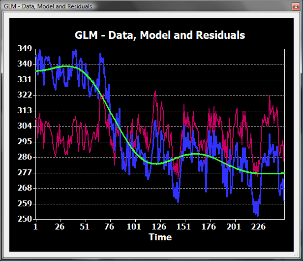
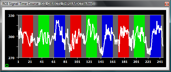
The following snapshot shows the result of the DCT GLM applied to the time course showing a non-linear drift. The obtained fit (green curve) looks very similar to the one obtained with the Fourier basis set.
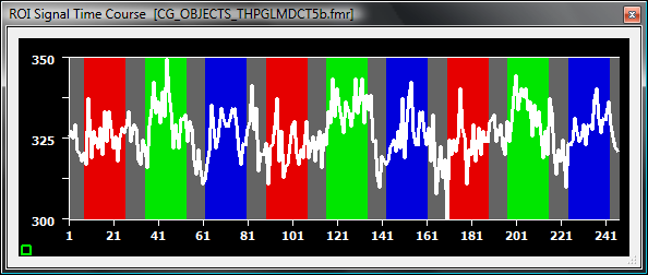
The magenta curve shows the difference between the blue and the green curve and serves as the new voxel's time course, which is the same as the time course below, which is from the same voxel of the DCT preprocessed FMR data. Again, the obtained result is very similar to the results obtained with the previous two methods.
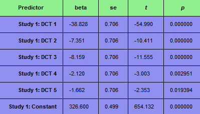
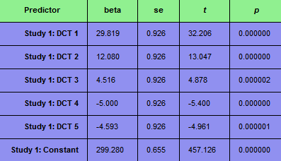
The beta values below indicate that the first DCT predictor is contributing the most in explaining the non-linear drift.
When the GLM DCT method is used for high-pass filtering, the name of the preprocessed FMR project will contain the substring "THPGLMDCT[N]b" (THP = temporal high-pass, GLM = general linear model, DCT = discrete cosine transform basis set, b = basis functions), where "[N]" will be replaced with the selected number of DCT predictors.
Summary and Conclusions
All three preprocessing approaches provide similar results effectively removing low frequency drifts in voxel time courses. While differences between methods are small, we have a small preference for the GLM-based Fourier analysis approach. While the selection of one of these methods is not very critical because all methods produce similar filtered data, it is important that the frequencies filtered out are below the frequencies contained in the stimulation protocol, otherwise the experimentally induced signal fluctuations will be removed from the data or at least strongly reduced. An important tool to check whether this is the case is described in topic High-Pass Filtering of Design Matrix. In order to demonstrate the effect of too much filtering, the following three time courses show the example voxel time course from above with the linear trend after filtering it with a Fourier basis set of 3, 6 and 9 cycles.
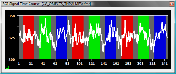
While the linear trend is removed in all cases, the high-pass filters remove an increasing amount of variability due to the stimulation blocks. While the filter with 3 cycles has only a minor effect, the filter with 6 cycles already reduces the stimulus-related variation substantially, which is almost completely removed after application of the filter with 9 cycles. This effect can be clearly seen when visualizing the GLM fit of the time course with the three different filters:
The 3 cycles filter removes only a small amount of signal variation. While the dominant block-related frequency is 9 cycles (9 blocks in time course), each individual condition appears only three times and may already affected by the filter.
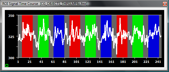
The filter with 6 cycles already removes a substantial amount of signal variation.

The filter with 9 cycles almost perfectly fits the block-related signal fluctuation (9 bumps) removing not only the linear trend but also the stimulus-related effects.
Copyright © 2023 Rainer Goebel. All rights reserved.